This is a quick guide to plotting curves using Tuva’s functioning editor, f(x). 

You can use the function editor to model the relationship between two quantitative attributes or variables.

The mechanics are simple—drag two quantitative attributes on the x and y axes, and fit a curve to approximate the relationship between the two attributes.

Step 1: Create the Scatterplot

Drag quantitative attributes to both the x and y axes.

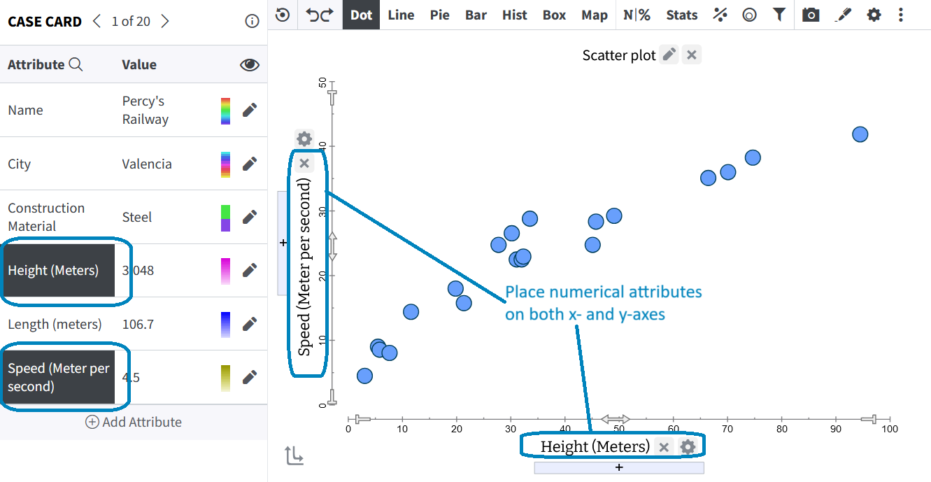Note: If you do not plot both an x and y attribute, the f(x) functionally will not allow you to plot a curve. 

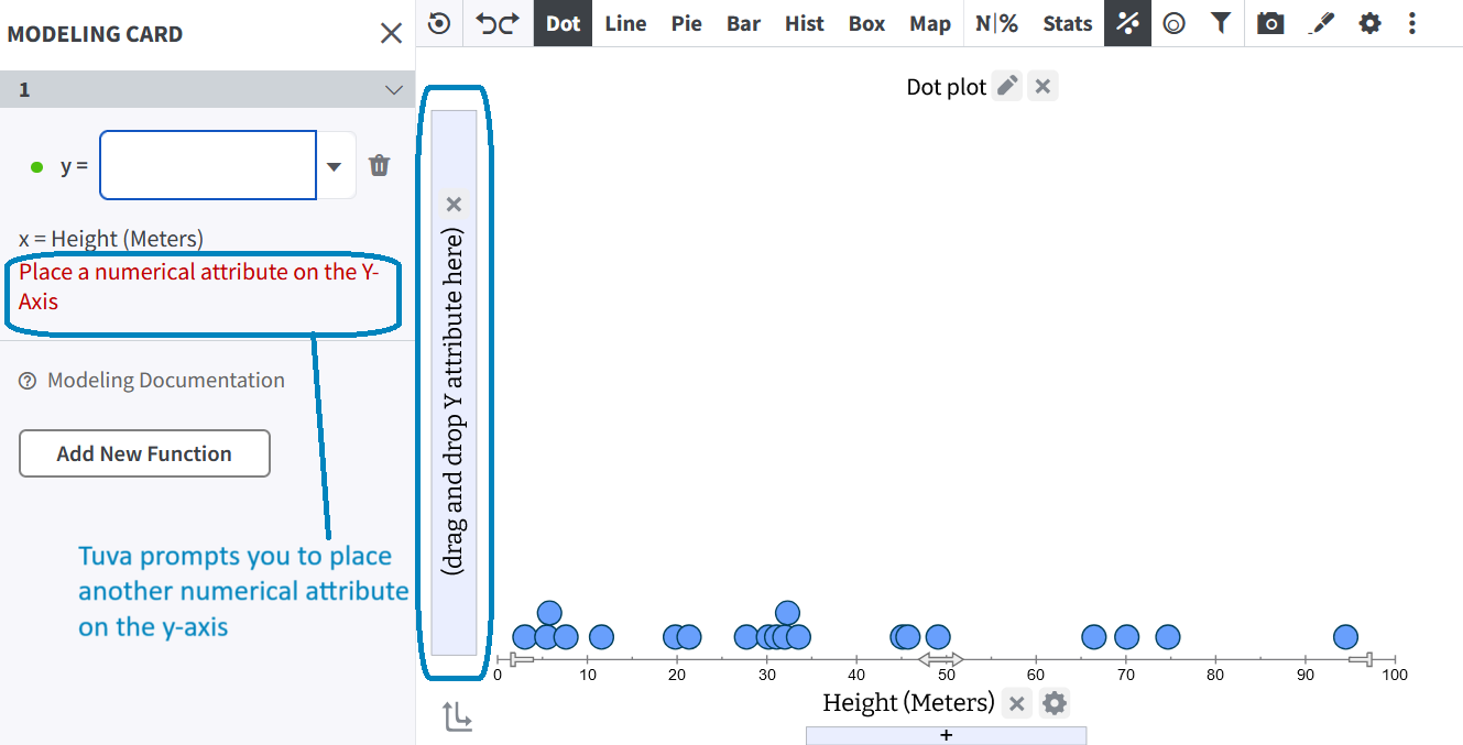Step 2: Open the Modeling Card

To model the relationship (which in this context is between roller coaster height and speed), click on Model Data on the toolbar. Next, choose f(x) from the dropdown to open the modeling card. The modeling card will appear on the left-hand side of your screen.

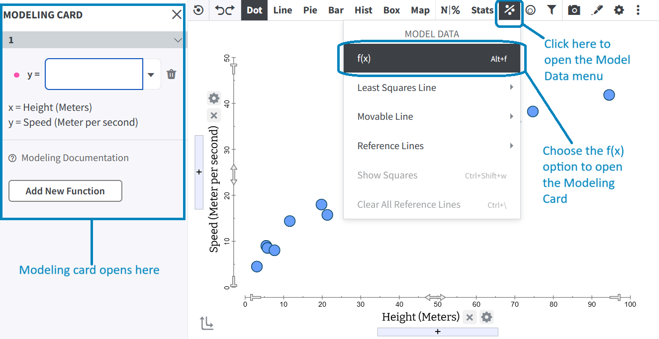Step 3: Form Your Function

In the modeling card, you can either enter the function in the editor or choose the desired function form from the drop-down menu. If you choose a function from the drop-down menu, you may need to adjust the function for your own context.   

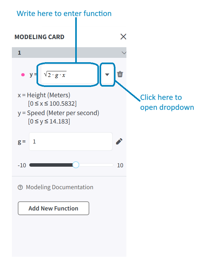When you have done this, two things happen:

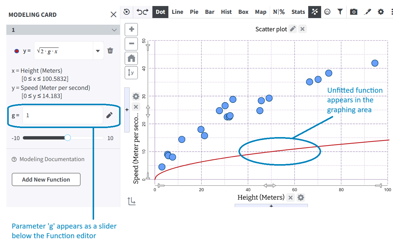
1. Your function will appear on the graph. If it doesn’t, you will need to estimate the range of the parameter to get it in the viewing window, and/or zoom out. See what to do when a function does not appear for more detailed instructions.

2. The parameter (g in this case) appears as a slider below the function editor in the modeling card.

Step 4: Tweak the Parameter

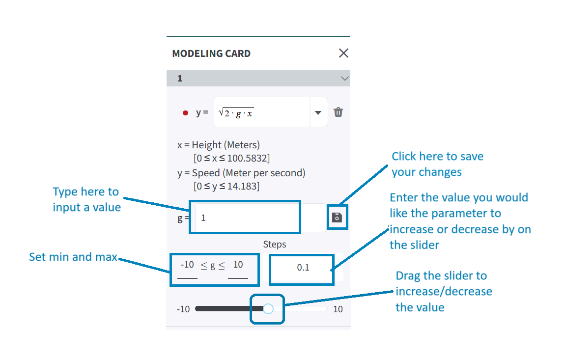
You can change the value of a parameter by dragging the slider pointer.  As you do this, the curve will move. Alternatively, you can type in a new value for the parameter and press enter. 

The default lower bound of the slider is -10 and the default upper bound is +10. You can tweak the minimum and maximum values by clicking on the edit icon adjacent to the parameter field and inputting the desired value. Once you are done, simply click the save button adjacent to the parameter field.

Additionally, if you feel that you need to make very small or large changes to the parameter value, input the desired value in the Steps field.

Try it Yourself! Practice tweaking the parameter on this dataset. See if you can find a good fit. (Note: You will need to open the modeling card by clicking f(x) from toolbar, as shown above). 

Step 5: Finding the Right Fit

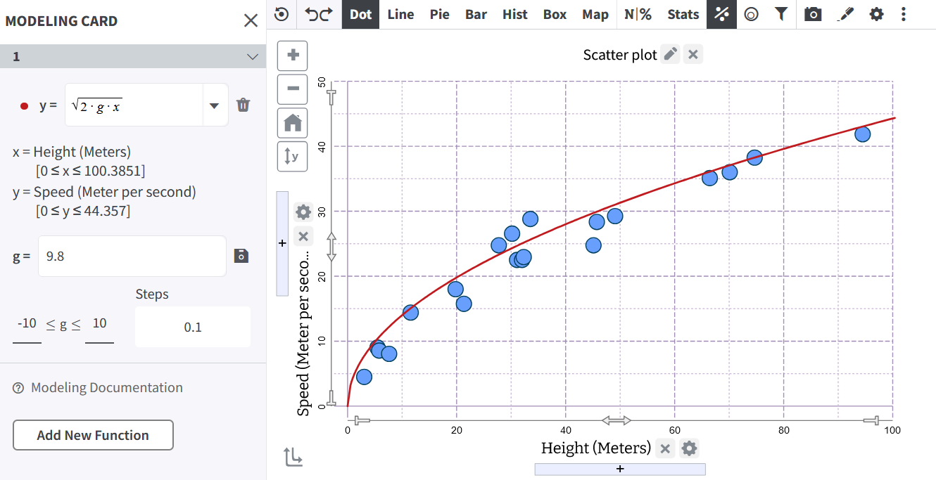
Continue to tweak the parameter value until you get the closest possible fit. In this case, you get a reasonable fit between 9.5 and 9.9.

Once you are happy with your fit, you are all set to start making sense of your function in the context of the data!